The Processed Data window presents the diagram described by the selected Function in the Data Organizer window.
Singular Value Decomposition
The Singular Value Decomposition or short SVD belongs in the group of Spectral density functions.
This display presents the singular values of the matrices of the estimated spectral density function. At each frequency there are as many singular values as there are measurements channels in the currently selected test setup or projection channels if enabled.
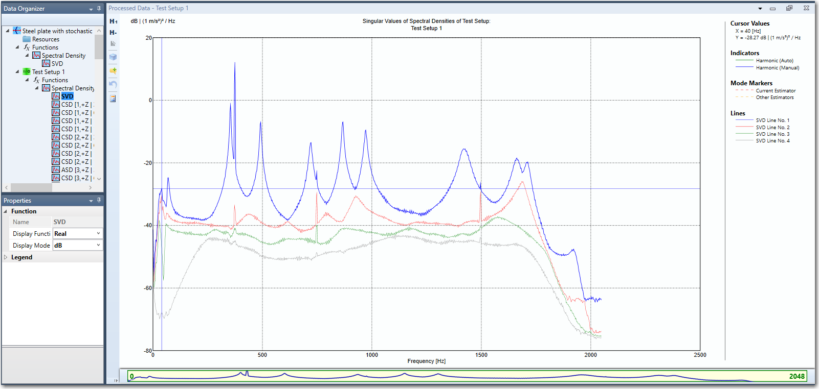
This display is a very useful tool because you can detect close modes, but also because the frequency content is presented in a single display. The singular value display show the rank of each of the spectral density matrices. If only one mode is dominating at a specific frequency only one singular value will be dominating at this frequency. If you have close or repeated modes you will see as many dominating singular values as there are close or repeated modes.
If a specific Test Setup has been selected in the Data Organizer the singular values presented are for this Test Setup. If the Measurement Project item is selected it will be an average of the singular values of all Test Setups that are displayed.
Spectral Density Magnitudes
The Spectral Density Magnitudes belong in the Spectral density Function Group. The short name from which the function can be identified in the data Organizer is CSD for Cross Spectral Densities and ASD for Auto Spectrl Densities.
If a specific Test Setup is selected this display presents the magnitude of the estimated spectral density function between two measurement channels as seen below.
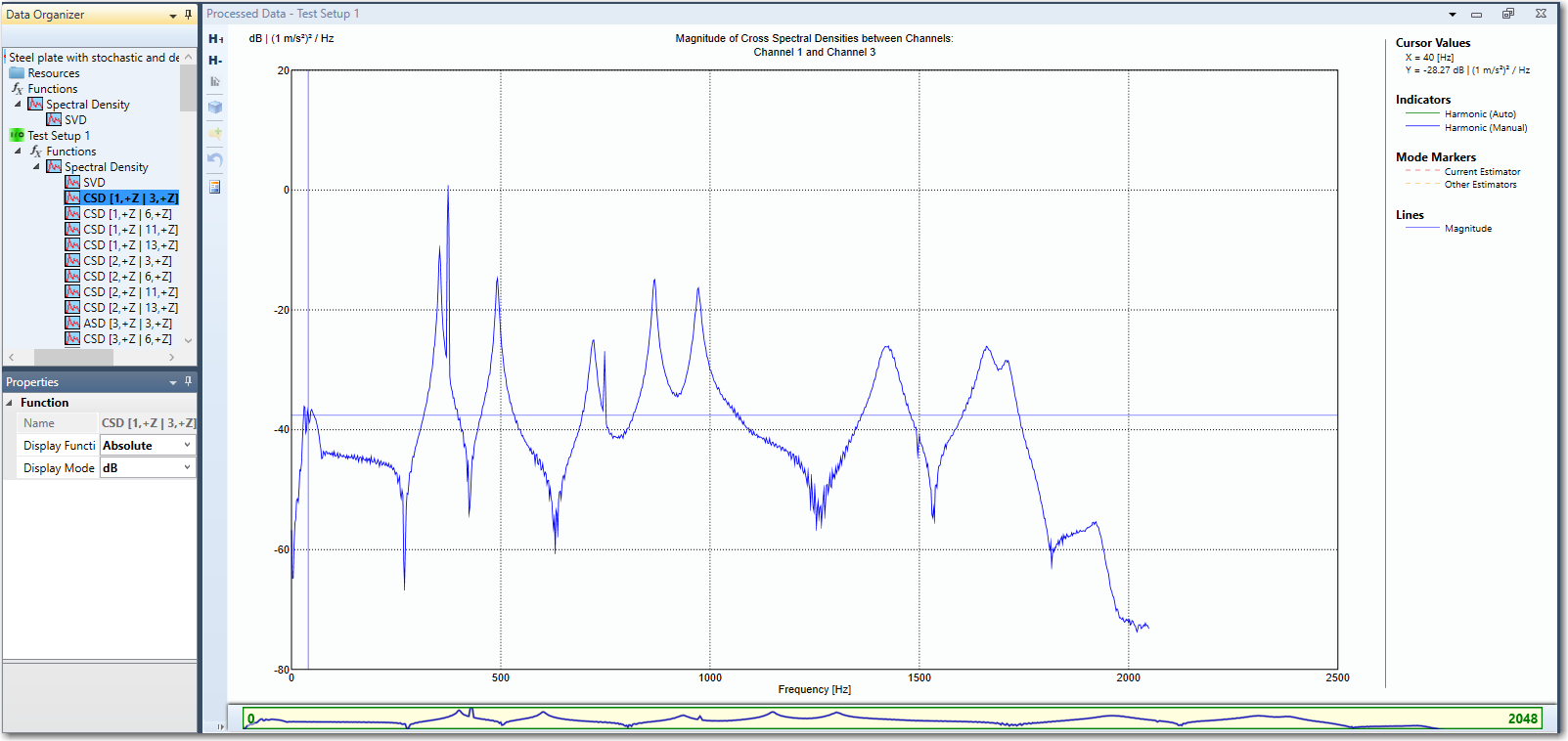
The cross spectral density being displayed is presented in the title of the view in terms of the labels of the channels and the currently selected test setup. I the Data Organizer there will be as many CSD functions as there are available channel combination. In the previous versions of the software this could be done from the Properties window, but starting from version 3.6 each CSD combination has it's own function item in the Data Organizer.
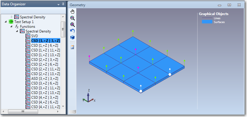
Note that while the Cross Spectral Densities are displayed in the Processed Data Window, the channels between which the CSD are calculated are also highlighted and blinking in the geometry window. This way the user can immediately see the sensors location.
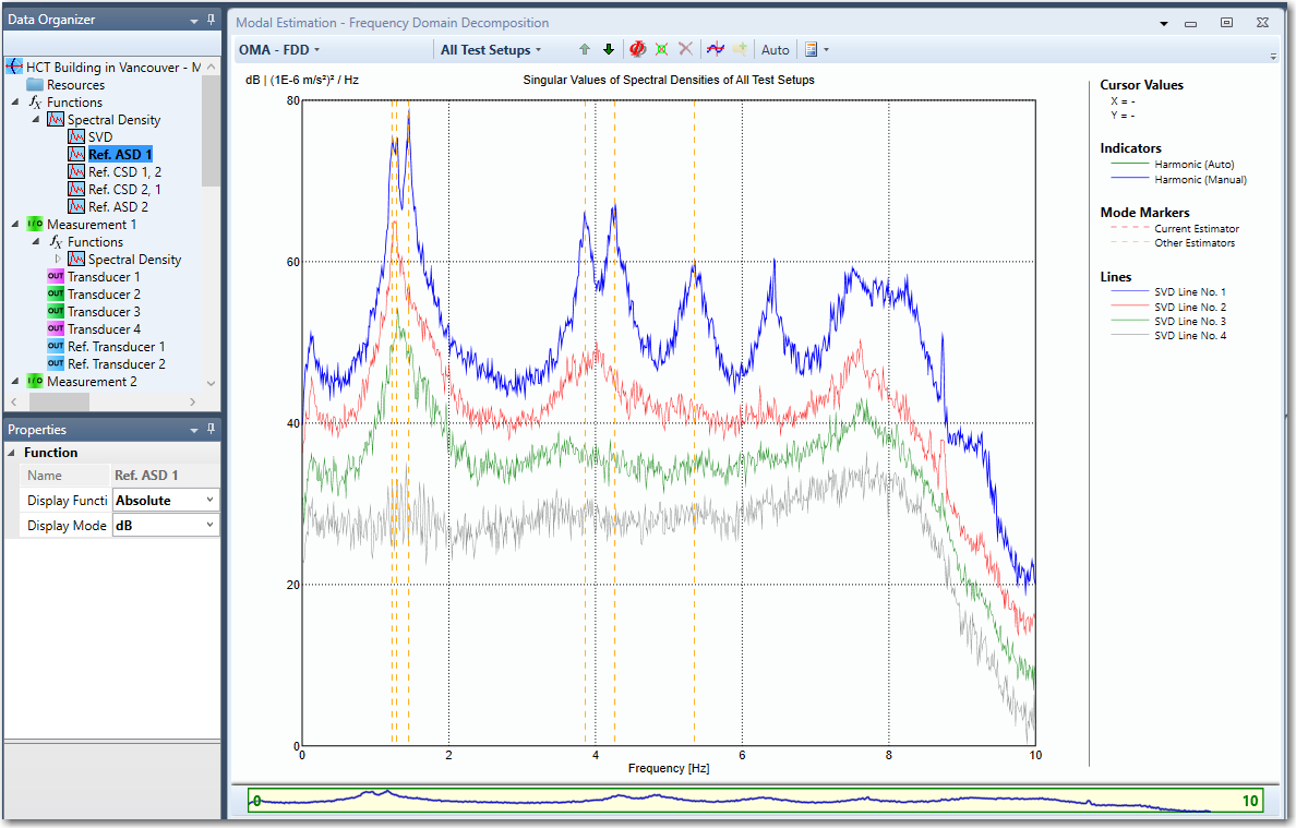
If the Measurement Project item is selected and if the project contains several Test Setups then the display will present the reference channels of the different Test Setups in the same diagram, see below:
Coherence
These functions can be identified in the Data Organizer by their short name Coh followed by the channels between which the Coherence of Cross Spectral Densities the function is presenting.
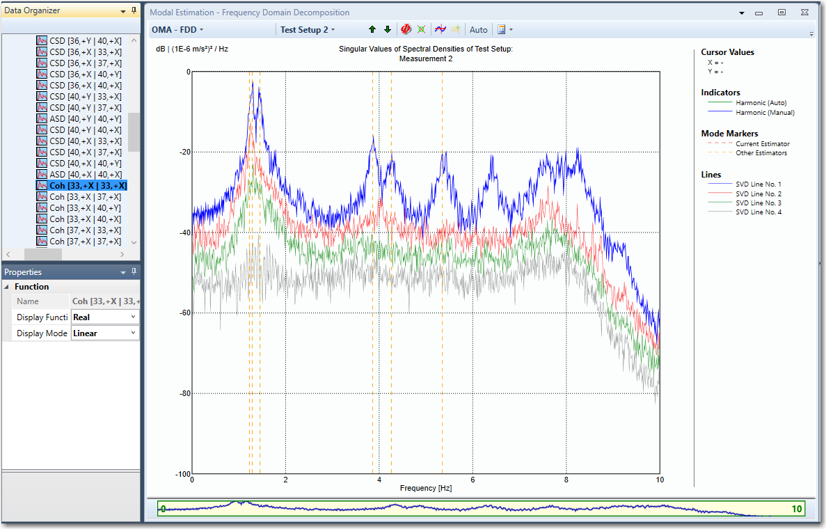
This display presents the coherence of the estimated spectral density function between two measurement channels. Please note that only the coherence between the reference transducers can be displayed when Measurement Project Item has been selected in the Data Organizer.
Average of Auto-spectral Densities
These functions can be identified in the Data Organizer by their short name Avg.
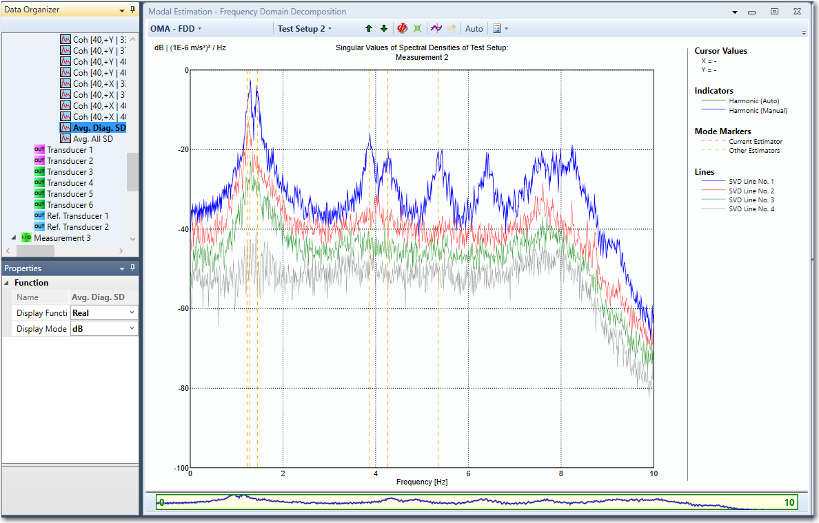
The average of auto-spectral densities provides a fast indication of where the most dominating modes are located and what the average energy level is.
Average of All Spectral Densities
These functions can be identified in the Data Organizer by their short name
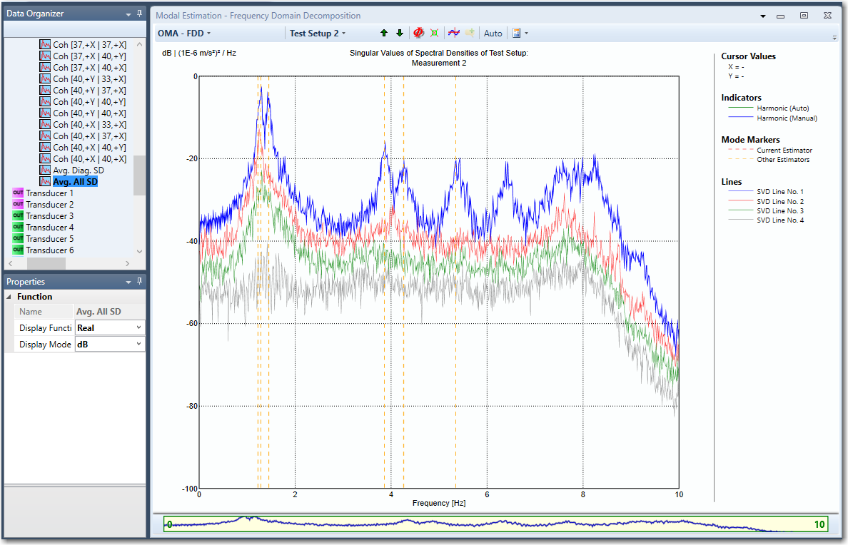
The average of all spectral densities provides a fast indication of where the most dominating modes are located and what the average energy level is.
Short Time Fourier Transform - STFT (Spectrogram)
The x-axis presents the frequencies between DC and the Nyquist frequency, The y-axis presents the measurement time. Red colors indicates the regions with most energy and dark blu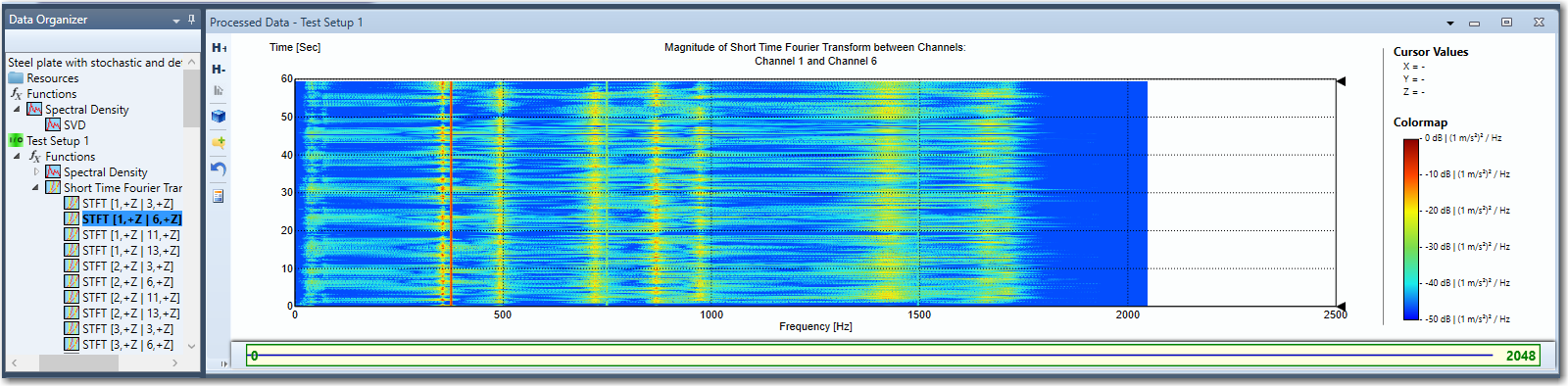
The x-axis presents the frequencies between DC and the Nyquist frequency, The y-axis presents the measurement time. Red colors indicates the regions with most energy and dark blue the regions with smallest energy level.
The average of the spectrogram (the squared STFT) in the time direction is called the frequency marginal. For some time-frequency distributions the frequency marginal actually equals the power spectrum (and the time marginal equals the signal squared), but this is not the case for the spectrogram, partly because of the positivity, and partly because of the inherent low pass filtering of the windowing used in creating the spectrogram. However, the frequency marginal resembles the power spectrum. Here the Power Spectral Density (PSD) is estimated using the Welch method, which is quite similar to the frequency marginal. To make the spectrogram similar in magnitude to the PSD, such as to enable a direct comparison between the two energy representations, the spectrogram has been modified so that the time-averaged value at any given frequency in the spectrogram has the same magnitude as the PSD for that frequency. Since the PSD is an estimated density where frequency resolution has been traded for better signal to noise ratio the same applies to the scaled spectrogram.
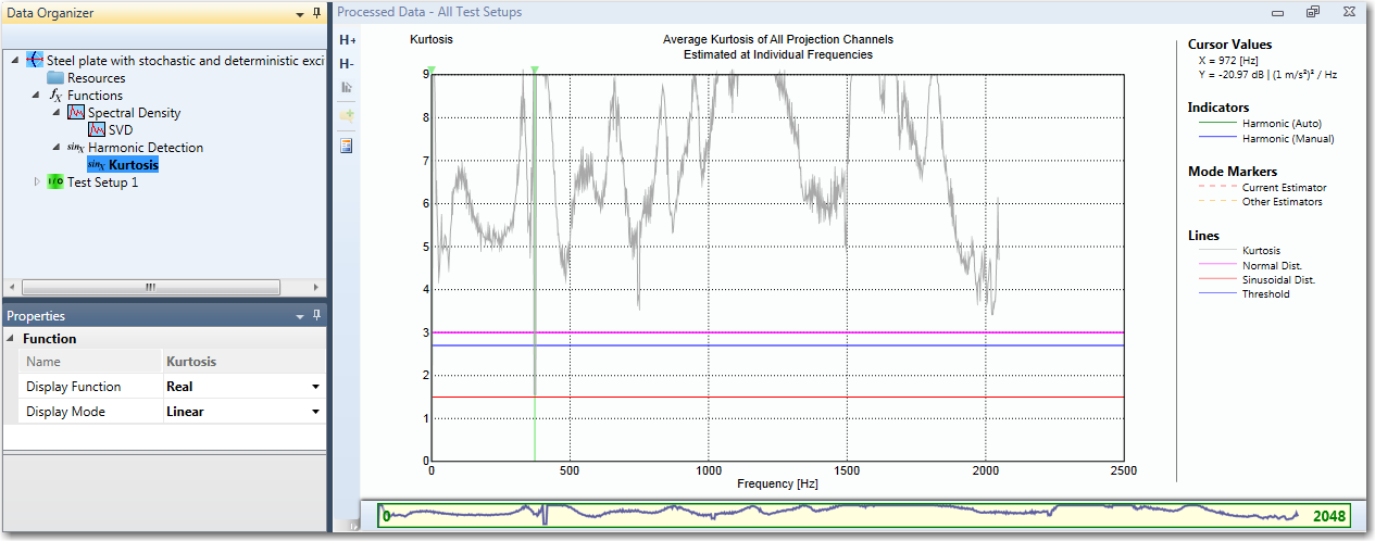
Average Kurtosis of All Projection Channels Estimated at Individual Frequencies
If there are spikes in more than one line in the Singular Value Decomposition diagram they most likely have their origin due to an harmonic excitation. These harmonics disturb the mode estimation and therefore it is preferable to detect and remove these harmonics from the mode estimation. To detect these harmonics you have to enable the harmonic detection in the Signal Processing window. When enabled and the measurements have been processed you are ready to detect the harmonics. After processing you can view the detected harmonics in all frequency domain windows by checking the Show Harmonic Indicators check box which can be found in the Properties window.
The consequences of having harmonic components present in the responses depend on both the nature of the harmonic components (number, frequency and level) and the modal parameter extraction method used. For the EFDD and CFDD techniques it is important that harmonic components inside the desired SDOF are identified and their influence eliminated before proceeding with the modal parameter extraction process. It should
be noticed that harmonic components cannot, in general, be removed by simple filtering as this would in most practical cases significantly change the poles of the structural modes and thereby their natural frequency and modal damping. So some other approach to eliminate the harmonics is needed.
The approach adopted here is based on the estimation of the statistical property called Kurtosis, which is the 4th order moment of the statistical distribution. The Kurtosis for a normal distribution with zero mean and unit variance is 3 and for a sine function with unit variance 1.5.
No matter if extended or fast harmonic checking is used, the mean values of the Kurtosis of all projection channels is calculated for all frequencies between 0 and the Nyquist frequency. To detect the harmonics in the frequency domain windows a threshold is used. The default value of this is 2.7, indicating that if at any frequency the Kurtosis drop below this value it is characterized as a harmonic. Since the Kurtosis only can be estimated and since the data can be far from normal distributed the default value of 2.7 might be either too small or large, in which case it can be adjusted in the Properties window.